The variation of molar conductivity with concentration of an electrolyte (X) in aqueous solution is shown in the given figure.

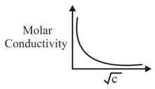
The electrolyte X is:

To identify the electrolyte represented by the given graph, we analyze the relationship between molar conductivity ($$\Lambda_m$$) and concentration.

The variation of molar conductivity with concentration is explained by Kohlrausch’s law and the Debye-Hückel-Onsager theory.

For strong electrolytes such as $$HCl$$, $$NaCl$$, and $$KNO_3$$, dissociation in solution is nearly complete. As the solution is diluted, the molar conductivity increases only gradually due to reduced interionic interactions. Consequently, the plot of $$\Lambda_m$$ versus $$\sqrt{c}$$ is almost linear and can be extrapolated to obtain the limiting molar conductivity, $$\Lambda_m^\circ$$.

In contrast, weak electrolytes such as $$CH_3COOH$$ undergo only partial dissociation. On dilution, the degree of dissociation increases significantly, causing a sharp rise in molar conductivity as the concentration approaches zero. As a result, the graph of $$\Lambda_m$$ versus $$\sqrt{c}$$ is distinctly non-linear and exhibits a steep upward curve.

The graph provided shows a pronounced, non-linear increase in molar conductivity with decreasing $$\sqrt{c}$$, which is the characteristic behavior of a weak electrolyte.

Among the given options:

• $$HCl$$ is a strong acid and dissociates completely.
• $$NaCl$$ is a strong electrolyte and dissociates completely.
• $$KNO_3$$ is a strong electrolyte and dissociates completely.
• $$CH_3COOH$$ is a weak acid and undergoes partial dissociation, producing the characteristic steep increase in molar conductivity upon dilution.

Hence, the electrolyte represented by the graph is

$$\boxed{CH_3COOH}.$$