Match the rate expressions in LIST-I for the decomposition of X with the corresponding profiles provided in LIST-II. $$X_s$$ and k constants having appropriate units.

LIST-I	LIST-II
(I) rate = $$\frac{k[X]}{X_s + [X]}$$, under all possible initial concentration of X	(P)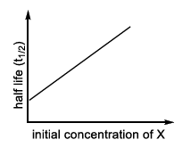
(II) rate = $$\frac{k[X]}{X_s + [X]}$$, where initial concentration of X are much less than $$X_s$$	(Q)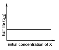
(III) rate = $$\frac{k[X]}{X_s + [X]}$$, where initial concentration of X are much higher than $$X_s$$	(R)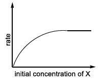
(IV) rate = $$\frac{k[X]^2}{X_s + [X]}$$, where initial concentration of X is much higher than $$X_s$$	(S)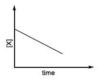
	(T)

The four rate expressions given in LIST-I resemble the Michaelis-Menten form that is often written for enzyme catalysis or surface-mediated (Langmuir-Hinshelwood) kinetics. In general, the rate of decomposition of $$X$$ is expressed as a function of its concentration $$[X]$$ and a saturation constant $$X_s$$.

$$\textbf{General form :}\qquad \text{rate}=\frac{k[X]^m}{X_s+[X]}$$
Here $$m=1$$ or $$2$$ depending on the mechanism.

To match each rate law with its graphical profile we analyse its limiting behaviour in the two extreme regimes:
(1) $$[X]\ll X_s$$ (very dilute substrate)
(2) $$[X]\gg X_s$$ (substrate present in large excess)

• When $$[X]\ll X_s$$, $$\;X_s+[X]\approx X_s\Rightarrow\text{rate}\approx\dfrac{k}{X_s}[X]$$ (first-order).
• When $$[X]\gg X_s$$, $$\;X_s+[X]\approx[X]\Rightarrow\text{rate}\approx k$$ (zero-order plateau).
Hence the plot of rate vs. $$[X]$$ rises linearly at first and then levels off to a constant value - the typical saturation (rectangular-hyperbola) curve. That overall curve is denoted in LIST-II by profile P.

Because the initial concentration is far smaller than $$X_s$$ we may replace $$X_s+[X]$$ by $$X_s$$ right from the start:
$$\text{rate}\approx\dfrac{k}{X_s}[X]$$
Thus the graph is a straight line through the origin whose slope is $$k/X_s$$ - a purely first-order dependence. In LIST-II that simple linear plot is labelled Q.

Now $$X_s+[X]\approx[X]$$, giving
$$\text{rate}\approx k\;(\text{independent of }[X])$$
Hence the rate is essentially constant; the profile is a horizontal line (zero-order region) tagged as S in LIST-II.

For very large $$[X]$$, $$X_s+[X]\approx[X]$$, so
$$\text{rate}\approx\frac{k[X]^2}{[X]}=k[X]$$
The rate once again varies linearly with concentration, but its slope is simply $$k$$ (different numerical value from Case II). The corresponding straight-line profile is marked T in LIST-II.

Collecting the matches:

I → P (general saturation curve)
II → Q (first-order straight line at low $$[X]$$)
III → S (zero-order plateau at high $$[X]$$)
IV → T (first-order straight line obtained from the $$[X]^2$$ law at high $$[X]$$)

Therefore, the correct option is:
Option A which is: I → P; II → Q; III → S; IV → T